Relational Algebra
Queries
Now that we can organize and store data, it’s time to query our data in interesting ways to answer questions
In order to manipulate our data, we need some sort of language to do this in
Luckily, Codd discussed this in his famous paper, giving us procedural languages (using relational algebra) and non-procedural languages (using relational calculus)
- Formally, relational algebra is equivalent to relational calculus, meaning we can convert between the two
For procedural languages, we’ll use SQL, which is the most popular
On top of SQL being relationally complete, we can do some other cool things like sorting and calculations
In order to talk more about SQL, we need to talk about relational algebra
Relational Algebra
Relational algebra is a language with operations that performs on relations and produces relations based on the operations
Since all our operations are relation → relation, this is a closed language, unlike division which isn’t (8/6 doesn’t give us an integer)
Since the language is closed, we can use output for one operation as input for another, the combination of which can be used for more complicated operations
- Ex. 3^4 = 3 x 3 x 3 x 3
In relational algebra, we have 5 basic operations
- Selection: returns the tuples that satisfy a condition, $\sigma_{condition}(R)$
- Projection: returns requested attributes (with no duplicates), i.e. a column subset, $\Pi_{attr_1, attr_2,…,attr_n}(R)$
- These are both unary operations
- Cartesian Product: returns the concatenation of every tuple in relation $R$ with every tuple in relation $S$, $R \times S$
- Union: returns the combination of two relations $R,S$, where their tuples $I,J$ are combined, $R \cup S$
- Set Difference: returns all tuples in relation $R$ but not in relation $S$, $R - S$
- SQL itself has operations that don’t produce closure, but relational algebra doesn’t
Let’s talk about each of these in more detail
Selection and Projection
Selection is pretty simple: collect all the tuples that meet a given condition
- For example, $\sigma_{age>30}(R)$ will return all tuples in $R$ where the attribute age > 30
Projection is also simple: collect all the attributes of a given name
- For example, $\Pi_{age, name}(R)$ will only give the age and name columns of the relation
We can combine these into other expressions as well, ex. $\Pi_{address}(\sigma_{gender=M}(R))$ gives only the addresses of men in the relation
- We could’ve split this operation as well
Sometimes we need to rename the attributes when doing union and joins, so we can change the names with a subscript
\[T_{2(addy)}\leftarrow \Pi_{address}(T_1)\]The order also matters (the sequence of operations below is invalid since gender doesn’t exist in $T_1$)
\[T_1 \leftarrow \Pi_{address}(R) \\ T_2 \leftarrow \sigma_{gender=M}(T_1)\]Duplicates rows are also not allowed in relation algebra, so we must remove them, which can cause some problems with projects depending on what we want to do
Union and Difference
In order to understand unions, we must talk about union compatibility
We say two relations are union compatible iff they have the same number of columns and each respective column in the same domain
For example, in the below diagram, TableA and TableB would not be union compatible, but TableB and TableD would
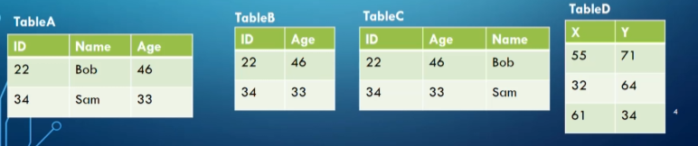
TableA and TableC wouldn’t work either since the respective columns don’t share domains
What $T_1\cup T_2$ does is create a table with rows of both $T_1$ and $T_2$ but with duplicates removed, assuming $T_1,T_2$ are union compatible
Difference also needs to be union compatible, however $T_1-T_2$ instead gives all rows that are in $T_1$ but not in $T_2$
Cartesian Product
The cartesian product $T_1 \times T_2$ maps every row in $T_1$ with every row in $T_2$, where $T_1,T_2$ aren’t necessarily union compatible
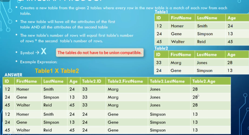
An example of what a cartesian product looks like
However, there is a restriction where the attributes can’t share names, so what we do is $”T_{name}.attr_{name}”$ for the names that are shared
The number of tuples in the resulting relation is the number of tuples in $T_1$ * the number of tuples in $T_2$, and the number of attributes is the number of attributes in $T_1$ + the number of attributes in $T_2$
When we combine cartesian product with what we know about foreign keys, what we can do now is match up every tuple with a tuple it’s associated with
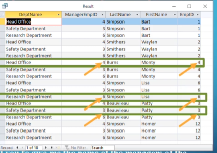
The cartesian product grabs every department manager next to the department they manage
From here, we can do $\Pi_{LastName, FirstName, DeptName}(\sigma_{ManagerEmpID=EmpID}(R))$ to get the names of all the department managers along with the department they manage
This effectively describes the join operation, which we’ll talk about now
Joins
Joins are what we described above, where we combine a cartesian product and a selection
- It looks like $T_1 \Join T_2$
There’s two main types of joins: inner and outer joins
Inner joins can be further divided into two subtypes: natural joins (where we only select for equivalence in the attributes that share names between each other) and equi joins (where we select for equivalence between two given attributes that share the same domain)
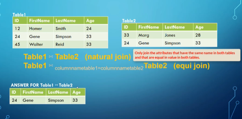
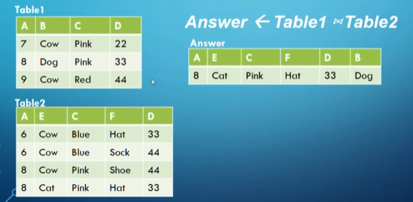
Natural join
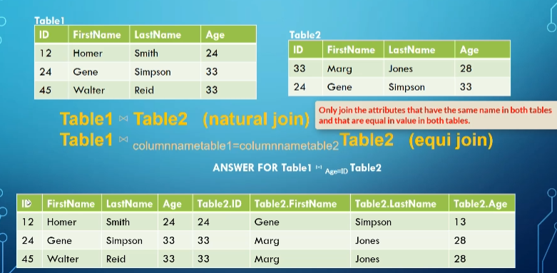
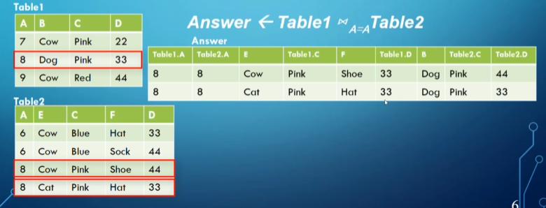
Equi join (we put the condition as a subscript)
For equi joins, we can use any boolean formula, meaning any formula with <, ≤, >, ≥, =, ≠, and, or, not
For a natural join, we include each pair of attributes with the same name ANDed together
\[Q \leftarrow R(A,B,C,D) \Join S(C,D,E) \\ R.C=S.C \text{ AND }R.D=S.D \\ Q(A,B,C,D,E)\]- This is opposed to equi join, which will match up within the boolean formula given and include all attributes of the cartesian product
- Remember that rows in a relation cannot be duplicates, this might trip you up on exams
If you want to join to use a many-to-many relationship, you have to use the relationship table as well
\[Employee \Join Works.On \Join Project\]Now we’ll talk about outer joins, which work slightly differently but still run on the same concept
Outer joins can be divided into three subtypes: full, left and right
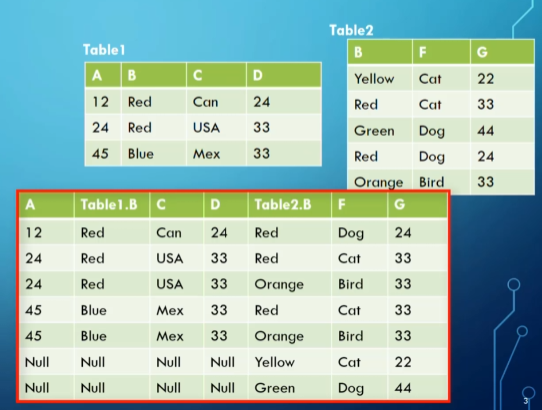
Full outer joins $T_1 \space ⟗ \space T_2$ include all rows from both tables at least once even if they don’t have a matching value
- If there’s no match, we put nulls in the columns from the other table
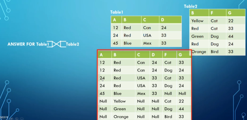
Notice the null values
We can also use conditions to make this an equi join in the same way we did for inner joins
We also have left joins, $R \space ⟕ \space S$ which include all the rows from $R$ but not necessarily from $S$
- Right join, $R \space ⟖ \space S$, works the same way but in reverse
Often we use outer joins when we want a full table but also additional related data from another table
For example, if we wanted to get every employee along with the name of the department they manage (if they manage one), we do something like this
\[T_1 \leftarrow Department \space ⟕_{ManagerEmpID=EmpID} \space Employee \\ A=\Pi_{FirstName, LastName, DeptName}(T_1)\]Intersection
Intersection is another one of our combination operations that returns only identical rows between two tables
\[R \cap S = (R \cup S)-((R-S)\cup(S-R))\]- $R,S$ must be union compatible, but I hope that’s obvious
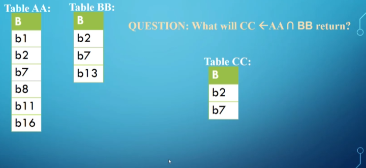
This is useful for any situation where you use ‘both’ or ‘and’, ex. get everyone who works on project A and project B
Division
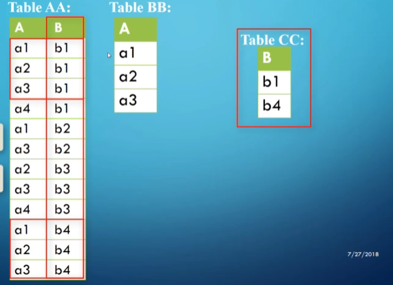
Division, $R \div S$, returns a new table that has only the columns that were in $R$ but not in $S$, as well as only the rows from the remaining columns of $R$ that match every row in $S$
- The columns of $S$ must be a subset of the columns in $R$
This is a bit complicated, so let’s look at an example
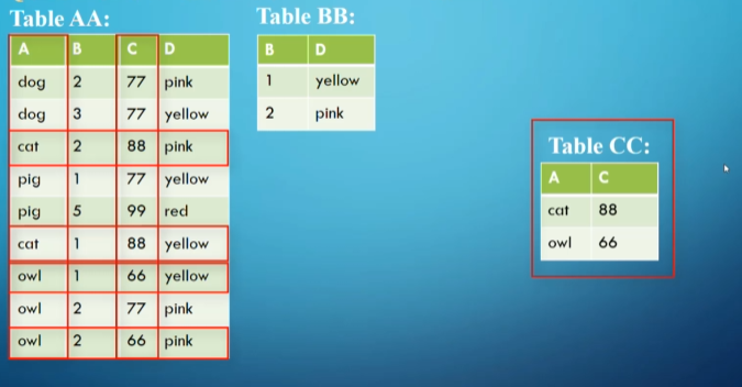
To see where this is useful, we can look at the following scenario
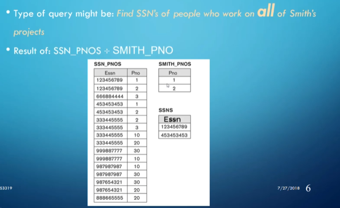
In general, when we have a scenario with the word ‘all’, we should look to division as the solution
- This is still not nearly as common as the other ones, but they still come up
To summarize everything we’ve learned so far:
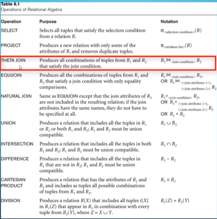
Theta join is effectively what we’ve been calling equijoins